How to Calculate P-Value

How to Calculate P-Value: A Complete Statistical Guide with Examples, Formulas, and Software Instructions

Understanding data requires more than looking at raw numbers. To make accurate, data-driven decisions, you must determine whether your results are statistically significant or simply a product of random chance. The p-value is the mathematical tool that answers that question with precision.

This guide shows you exactly how to calculate the p-value manually, in Excel, on a TI-84 calculator, and using statistical software. Whether you are a student writing a research paper, a data scientist running A/B tests, or a business analyst evaluating campaign performance, this resource covers every method you need. Try the Calculator:

What Is a P-Value? Definition and Core Concepts

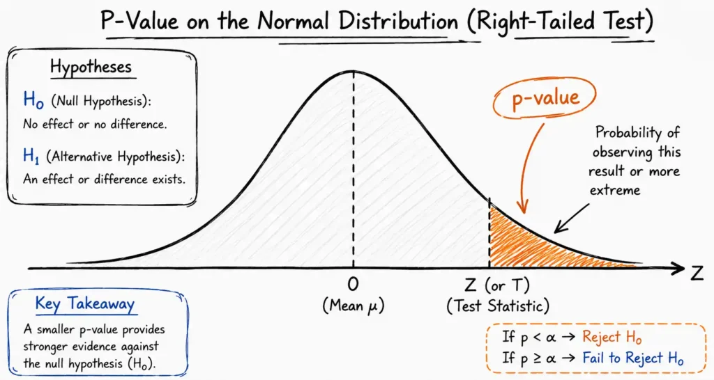
A p-value, short for probability value, is a number between 0 and 1 that describes how likely your observed data would occur purely by random chance, assuming your baseline assumption is true.

More precisely, the p-value answers this question: If nothing is actually different in the real world, how often would I see data this extreme or more extreme purely by luck?

A low p-value signals that your data is highly unusual under the assumption that nothing changed. A high p-value suggests the data is consistent with pure randomness.

The p-value does not measure the size of an effect. It does not tell you the probability that your hypothesis is true. It only tells you how surprising your observed data is if the null hypothesis were true.

Why P-Values Matter in Research and Business

Without p-values, researchers and businesses would constantly chase false positives. A marketing team might spend months optimizing a webpage change that produced a temporary statistical fluke. A pharmaceutical company might advance a drug that works no better than a sugar pill.

According to a 2019 statement published in Nature, over 800 statisticians and scientists called for a more careful interpretation of p-values, highlighting their importance and frequent misuse across scientific fields. The p-value remains the global standard for statistical decision-making when used correctly alongside effect sizes and confidence intervals.

Who Should Use This Guide

• Students mastering statistical analysis for coursework and exams
• Data scientists validating machine learning models and feature selection
• A/B testing marketers confirming whether a design change truly increases conversions
• Healthcare researchers proving whether a treatment outperforms a placebo
• Business analysts making evidence-based operational decisions

The Core Pillars of Hypothesis Testing: Null vs. Alternative

Before you calculate any p-value, you must build a formal statistical framework. This framework rests on two competing statements and one decision threshold.

Defining the Null Hypothesis (H0)

The null hypothesis (H0) represents the status quo. It states that there is no effect, no difference, or no meaningful relationship between your variables. It is the assumption you treat as true until your data proves otherwise.

Example: A bakery claims its loaves weigh exactly 500 grams. The null hypothesis states that the true average weight equals 500 grams.

Defining the Alternative Hypothesis (Ha)

The alternative hypothesis (Ha), also written as H1, is the claim you want to prove. It states that a meaningful effect, a significant difference, or a clear relationship exists between the variables you are testing.

Example: The alternative hypothesis states the true average weight is not 500 grams.

Choosing Your Significance Level (Alpha)

The significance level (alpha, or α) is the threshold you set before running your test. It represents the maximum risk you accept of committing a Type I error, which means rejecting the null hypothesis when it is actually true.

Standard alpha levels used across industries include:

Alpha Level	Percentage	Common Use Case
α = 0.05	5%	General research, business analytics, marketing
α = 0.01	1%	Manufacturing quality control, financial modeling
α = 0.001	0.1%	Clinical trials, pharmaceutical safety studies

The most widely used threshold is α = 0.05, set as a convention by statistician Ronald Fisher in the 1920s and adopted globally as the standard benchmark.

Type I and Type II Errors Explained

Every hypothesis test carries two types of possible mistakes.

A Type I error (false positive) occurs when you reject the null hypothesis even though it is actually true. The alpha level directly controls this risk. Setting α = 0.05 means you accept a 5% chance of this error.

A Type II error (false negative) occurs when you fail to reject a false null hypothesis. The probability of a Type II error is called Beta (β). Statistical power, defined as 1 − β, represents your test’s ability to correctly detect a real effect when one exists.

Larger sample sizes reduce both error rates simultaneously and increase the statistical power of your test.

Step-by-Step Guide to Calculating P-Value Manually

To find a p-value by hand, you must follow a structured series of mathematical steps. Skipping any step produces unreliable results.

Step 1: State Your Hypotheses Clearly

Write down your H0 and Ha before collecting or analyzing any data. Changing your hypotheses after seeing the data is a form of p-hacking and invalidates your conclusions.

Example: You test whether a new training program improves employee productivity scores.

• H0: The new program has zero effect on productivity scores (mean difference = 0)
• Ha: The new program improves productivity scores (mean difference > 0)

Step 2: Choose the Correct Statistical Test

Your test selection depends on your sample size and data structure.

• Use a Z-test when your sample size is large (n ≥ 30) and you know the population standard deviation (sigma)
• Use a t-test when your sample size is small (n < 30) or the population standard deviation is unknown
• Use a Chi-Square test when you are analyzing categorical data from a contingency table

Step 3: Calculate the Test Statistic

The test statistic measures how far your sample result deviates from the null hypothesis value. It converts raw data into a standardized score.

Z-Test Formula:

Z = (x-bar − mu) / (sigma / square root of n)

Where:

• x-bar = Sample mean
• mu = Population mean stated in the null hypothesis
• sigma = Known population standard deviation
• n = Sample size

T-Test Formula:

t = (x-bar − mu) / (s / square root of n)

Where:

• s = Sample standard deviation (used when sigma is unknown)
• Degrees of freedom (df) = n − 1

Step 4: Determine the Degrees of Freedom

Degrees of freedom (df) represent the number of independent values that can vary in your calculation. This parameter shapes the t-distribution curve and controls how heavy the tails of the distribution are.

For a single-sample t-test: df = n − 1

For a two-sample t-test: df = n1 + n2 − 2

For a Chi-Square test: df = (rows − 1) × (columns − 1)

As the degrees of freedom increase, the t-distribution curve approaches the shape of a standard normal (Z) distribution.

Step 5: Map the Statistic to the P-Value

Once you have your Z-score or t-score, convert it to a p-value using one of these methods:

• Standard statistical table: Look up the corresponding probability in a printed Z-table or t-distribution table
• Graphing calculator: Use built-in statistical test functions (see the TI-84 section below)
• Spreadsheet software: Use built-in functions in Excel or Google Sheets (see the Excel section below)

The p-value equals the area under the probability distribution curve that lies beyond your calculated test statistic.

Step 6: Make Your Statistical Decision

Compare your calculated p-value to your pre-set alpha level:

• If p-value < alpha: Reject the null hypothesis. Your results are statistically significant.
• If p-value ≥ alpha: Fail to reject the null hypothesis. Your results are not statistically significant.

Important: “Fail to reject” does not mean the null hypothesis is true. It means your data did not provide strong enough evidence to disprove it.

How to Calculate P-Value in Microsoft Excel

Excel contains several built-in statistical functions that calculate p-values directly from your raw data or test statistics. No manual table lookup is required.

Using T.TEST for a T-Test P-Value

The T.TEST function in Excel calculates the p-value for a two-sample t-test comparing the means of two datasets.

Syntax:

=T.TEST(array1, array2, tails, type)

• array1: The first column or range of data values
• array2: The second column or range of data values
• tails: Enter 1 for a one-tailed test, or 2 for a two-tailed test
• type: Enter 1 for a paired t-test, 2 for a two-sample equal-variance test, or 3 for a two-sample unequal-variance test

Step-by-Step Example in Excel:

1. Enter your first dataset in column A (for example, cells A2 through A11)
2. Enter your second dataset in column B (cells B2 through B11)
3. Click on an empty cell where you want the p-value to appear
4. Type: =T.TEST(A2:A11, B2:B11, 2, 3)
5. Press Enter to display the two-tailed p-value

Using NORM.S.DIST for a Z-Test P-Value

When you already have a calculated Z-score, use NORM.S.DIST to find the p-value from the standard normal distribution.

Syntax for a one-tailed p-value:

=1 - NORM.S.DIST(z_score, TRUE)

Syntax for a two-tailed p-value:

=2 * (1 - NORM.S.DIST(ABS(z_score), TRUE))

For example, if your Z-score is 2.35, enter =2*(1-NORM.S.DIST(2.35,TRUE)) to get the two-tailed p-value of approximately 0.0188.

Using Z.TEST for a Full Z-Test

The Z.TEST function performs a complete one-tailed Z-test on a dataset directly.

Syntax:

=Z.TEST(array, x, sigma)

• array: Your sample data range
• x: The hypothesized population mean (H0 value)
• sigma: The known population standard deviation (if omitted, Excel uses the sample standard deviation)

Using CHISQ.TEST for a Chi-Square P-Value

For categorical data analysis, the CHISQ.TEST function compares observed counts to expected counts.

Syntax:

=CHISQ.TEST(actual_range, expected_range)

Enter your observed frequency counts in one cell range and your expected frequency counts in a second cell range. Excel automatically calculates the Chi-Square statistic and returns the p-value directly.

Pro Tip: Always double-check that your data range selections match exactly between the two arrays in CHISQ.TEST. A mismatched range size returns an error.

How to Find P-Value on a TI-84 Calculator

The TI-84 Plus graphing calculator has a built-in TESTS menu that performs complete hypothesis tests and returns the p-value without any manual formula work.

Running a Z-Test on the TI-84

Follow this exact button sequence:

1. Press the STAT button
2. Press the right arrow key to navigate to the TESTS submenu
3. Select 1: Z-Test
4. Choose Stats (if you are entering summary statistics) or Data (if you have entered raw data in a list)
5. Enter the required values:
   • mu0: The null hypothesis population mean
   • sigma: The known population standard deviation
   • x-bar: Your sample mean
   • n: Your sample size
6. Select the direction of your alternative hypothesis (not equal, less than, or greater than)
7. Scroll down and select Calculate
8. The screen displays the Z-score and the p-value directly

Running a T-Test on the TI-84

1. Press the STAT button
2. Navigate to the TESTS submenu
3. Select 2: T-Test
4. Choose Stats or Data
5. Enter:
   • mu0: The null hypothesis population mean
   • x-bar: Your sample mean
   • Sx: Your sample standard deviation
   • n: Your sample size
6. Select the direction of your alternative hypothesis
7. Select Calculate
8. The screen displays the t-statistic, degrees of freedom, and p-value

Running a Chi-Square Test on the TI-84

1. Enter your observed values into Matrix A using 2nd → MATRIX → EDIT → [A]
2. Press the STAT button and navigate to TESTS
3. Select C: χ²-Test
4. Confirm the observed matrix is [A] and the expected matrix is [B]
5. Select Calculate
6. The screen displays the Chi-Square statistic and the p-value

Calculating P-Values for Chi-Square Tests

The Chi-Square test measures whether observed frequencies in categorical data differ significantly from expected frequencies. It is widely used in surveys, quality control, genetics, and market research.

The Chi-Square Test Statistic Formula

Chi-Square = Sum of [(Observed − Expected)^2 / Expected]

This calculation is performed for every cell in your contingency table, and the results are summed together.

Degrees of freedom for a Chi-Square test of independence:

df = (number of rows − 1) × (number of columns − 1)

Example: A clothing retailer surveys 200 customers across two store locations to see whether product preferences (T-shirts or Hoodies) differ by location.

	T-Shirts	Hoodies	Row Total
Location A	60 (Observed)	40 (Observed)	100
Location B	50 (Observed)	50 (Observed)	100
Column Total	110	90	200

Expected value for each cell = (Row Total × Column Total) / Grand Total

• Expected: Location A / T-Shirts = (100 × 110) / 200 = 55
• Expected: Location A / Hoodies = (100 × 90) / 200 = 45
• Expected: Location B / T-Shirts = (100 × 110) / 200 = 55
• Expected: Location B / Hoodies = (100 × 90) / 200 = 45

Chi-Square = [(60−55)^2/55] + [(40−45)^2/45] + [(50−55)^2/55] + [(50−45)^2/45]

Chi-Square = [25/55] + [25/45] + [25/55] + [25/45]

Chi-Square = 0.455 + 0.556 + 0.455 + 0.556 = 2.02

With df = (2−1) × (2−1) = 1, a Chi-Square statistic of 2.02 yields a p-value of approximately 0.155. Because 0.155 > 0.05, there is no statistically significant difference in product preference between the two locations.

Interpreting P-Values: What P < 0.05 Really Means

The most critical skill in statistics is correctly interpreting a p-value. Misinterpretation is common even among experienced professionals.

The Rule: P-Value vs. Alpha

The decision rule is simple:

• P < α (for example, p < 0.05): The evidence against the null hypothesis is strong enough to reject it. Results are statistically significant.
• P ≥ α: The evidence is insufficient to reject the null hypothesis. Results are not statistically significant.

What P < 0.05 Actually Means

A p-value of 0.05 means there is a 5% probability of observing a test statistic as extreme as your result, or more extreme, if the null hypothesis were completely true.

It does not mean:

• There is a 95% probability that your hypothesis is correct
• The result is large or practically important
• The null hypothesis is false with 95% confidence

The Relationship Between Alpha, Beta, and Statistical Power

Term	Symbol	Definition
Significance Level	α	Probability of a Type I error (false positive)
Type II Error Rate	β	Probability of a Type II error (false negative)
Statistical Power	1 − β	Probability of detecting a real effect when it truly exists
P-Value	p	Calculated probability from your observed sample data

A well-powered study (power ≥ 0.80) means there is at least an 80% chance of detecting a true effect. Achieving high power requires a sufficiently large sample size, determined before data collection through a power analysis.

Setting α = 0.05 means accepting a 5% risk of a false positive. To reduce both error types simultaneously, researchers increase their sample size before the experiment begins.

Calculator Guide: Inputs, Outputs, and Assumptions

An online p-value calculator simplifies the entire calculation. To get accurate results, you must understand exactly what each input field requires and what each output means.

Required Inputs

Input Field	What to Enter	Notes
Test Statistic (Z or t)	The numerical score from Step 3	Enter the full decimal value including sign
Degrees of Freedom (df)	n − 1 for one-sample t-tests	Only required for t-tests, not Z-tests
Test Direction	One-tailed or two-tailed	Based on your alternative hypothesis direction
Significance Level	0.05, 0.01, or 0.001	Enter your pre-selected alpha level

Understanding the Outputs

One-Tailed P-Value: The probability of getting a result as extreme as yours in one specific direction (greater than or less than). Use this when your alternative hypothesis specifies a direction.

Two-Tailed P-Value: The probability of getting a result as extreme as yours in either direction. Use this when your alternative hypothesis simply states “not equal to” without specifying direction. The two-tailed p-value is always exactly double the one-tailed p-value.

Statistical Decision: A direct output stating whether to reject or fail to reject the null hypothesis based on your entered alpha level.

Assumptions and Limitations

Calculators and formulas rely on several mathematical assumptions:

• Random sampling: Your data was collected through a genuine random process, not convenience sampling
• Normal distribution: The underlying population follows an approximately normal distribution (or your sample size is large enough for the Central Limit Theorem to apply)
• Independence: Each observation in your dataset is independent of every other observation
• No extreme outliers: Significant outliers distort the test statistic and produce unreliable p-values

If your data violates these assumptions, consider non-parametric alternatives such as the Mann-Whitney U test or the Kruskal-Wallis test.

Real-World Examples: Z-Test and T-Test Walkthroughs

Example 1: E-Commerce A/B Testing (Z-Test)

An online retailer wants to determine whether a red checkout button increases the average order value compared to the current blue button. Historical data shows a population mean order value of $50 with a known population standard deviation of $10.

Test Setup:

• Sample size (n): 100 shoppers
• Sample mean (x-bar): $53
• H0: The true mean = $50 (no improvement)
• Ha: The true mean > $50 (one-tailed, testing for increase only)
• Alpha: 0.05

Step 1 — Calculate the Z-score:

Z = (53 − 50) / (10 / square root of 100)

Z = 3 / (10 / 10)

Z = 3 / 1 = 3.0

Step 2 — Find the p-value:

A Z-score of 3.0 corresponds to a one-tailed p-value of 0.0013.

Step 3 — Decision:

Because 0.0013 < 0.05, the retailer rejects the null hypothesis. The red button produces a statistically significant increase in average order value.

In Excel: =1 - NORM.S.DIST(3.0, TRUE) returns 0.0013.

Practical note: The average order value increased by $3. Before launching the red button site-wide, the team should confirm that a $3 increase justifies the design and development cost — this is a question of practical significance, not statistical significance.

Example 2: Small Batch Manufacturing Quality Control (T-Test)

A boutique coffee roaster claims their bags contain exactly 12 ounces of coffee beans. A quality control inspector pulls a small random sample to verify this claim.

Test Setup:

• Sample size (n): 10 bags
• Degrees of freedom (df): 10 − 1 = 9
• Sample mean (x-bar): 11.8 ounces
• Sample standard deviation (s): 0.3 ounces
• H0: The true mean = 12 ounces
• Ha: The true mean ≠ 12 ounces (two-tailed test)
• Alpha: 0.05

Step 1 — Calculate the t-statistic:

t = (11.8 − 12) / (0.3 / square root of 10)

t = (−0.2) / (0.3 / 3.162)

t = (−0.2) / 0.0949

t = −2.11

Step 2 — Find the p-value:

Using a t-distribution table with df = 9, a two-tailed t-statistic of −2.11 yields a p-value of approximately 0.064.

Step 3 — Decision:

Because 0.064 > 0.05, the inspector fails to reject the null hypothesis. There is not enough statistical evidence to conclude the roaster is underfilling the bags.

In Excel: =T.TEST(data_range, reference_value, 2, 1) or use =T.DIST.2T(ABS(-2.11), 9) which returns approximately 0.064.

Practical note: The inspector might consider increasing the sample size to 30 or 40 bags to improve statistical power. With only 10 bags and a p-value of 0.064, there is a meaningful chance the roaster is genuinely underfilling but the small sample could not detect it with enough certainty.

Statistical Method Comparisons: Choosing the Right Test

Selecting the wrong test invalidates your entire analysis. Use the comparison tables below to guide every decision.

One-Tailed vs. Two-Tailed Tests

Feature	One-Tailed Test	Two-Tailed Test
Direction	Tests for an effect in one specific direction (greater than or less than)	Tests for any difference, regardless of direction
When to Use	When a change in the opposite direction is impossible or irrelevant	When any deviation from the baseline matters
Statistical Power	Higher power to detect an effect in the chosen direction	Lower power because alpha is split across both tails
Example Ha	“The new drug reduces blood pressure”	“The new drug changes blood pressure”
P-value relationship	P-value equals the one-tailed area	P-value equals double the one-tailed area

Z-Test vs. T-Test: Selection Matrix

Criterion	Use a Z-Test	Use a T-Test
Sample Size	Large (n ≥ 30)	Small (n < 30)
Population Standard Deviation	Known (sigma is given)	Unknown (estimate using sample s)
Distribution Shape	Assumes standard normal curve	Uses wider tails to account for uncertainty
Typical Application	National election polling, website traffic analysis	Lab experiments, small product batches, clinical pilots
Software Function (Excel)	NORM.S.DIST or Z.TEST	T.TEST or T.DIST

Choosing Between t-Test, Z-Test, Chi-Square, and ANOVA

Scenario	Recommended Test
Comparing means, large sample, known sigma	Z-Test
Comparing means, small sample or unknown sigma	T-Test
Analyzing categorical frequency data	Chi-Square Test
Comparing means across three or more groups	One-Way ANOVA
Comparing two related measurements (before/after)	Paired T-Test

Adjusting P-Values for Multiple Comparisons: The Bonferroni Correction

When researchers run multiple hypothesis tests on the same dataset simultaneously, the probability of at least one false positive increases rapidly. This problem is known as Type I error inflation or the multiple comparisons problem.

For example, if you run 20 separate tests each with α = 0.05, the probability of observing at least one false positive by pure chance is approximately 1 − (0.95)^20 = 0.64, meaning a 64% chance of a spurious result.

Applying the Bonferroni Correction

The Bonferroni correction adjusts the required significance level downward based on the number of tests performed.

Adjusted alpha = Original alpha / Number of comparisons

Example: If you test five different price points simultaneously and set α = 0.05:

Adjusted alpha = 0.05 / 5 = 0.01

Each individual test must achieve a p-value below 0.01, not 0.05, to be considered statistically significant after the correction.

The Bonferroni correction is conservative. When you are running a very large number of tests (hundreds or thousands), consider the Benjamini-Hochberg procedure instead, which controls the false discovery rate rather than the family-wise error rate and produces more statistical power.

Common Pitfalls: P-Hacking and Practical Significance

Misinterpreting p-values is one of the most pervasive errors in modern research, marketing, and data science.

Warning: P-Hacking Destroys Research Credibility

P-hacking (also called data dredging or data fishing) occurs when researchers run multiple statistical tests on the same dataset, try different subgroups, remove outliers selectively, or adjust hypotheses until they find a result with p < 0.05.

This practice inflates false positives and makes published findings unreliable. A 2015 analysis published in Science estimated that only 36% of social science studies reproduced their original statistically significant findings when independently repeated.

P-Hacking Prevention Checklist:

Before publishing or acting on results, ask yourself:

1. Was my hypothesis stated in writing before any data was collected?
2. Was my sample size determined by a power analysis before the experiment began?
3. Did I avoid removing data points after seeing their effect on the p-value?
4. Did I run only the pre-specified tests, not additional tests to find significance?
5. Am I reporting all tests I ran, including those with non-significant results?

If you cannot answer yes to all five questions, your p-value may not be reliable.

The Misconception of Practical Significance

A very small p-value does not mean your result is large, important, or actionable. It only means you are confident the result did not arise by random chance.

Consider this scenario: A technology company tests a new algorithm across 5 million users. Even a one-millisecond improvement in page load time might yield a p-value well below 0.001, making it highly statistically significant. But does saving one millisecond justify six months of engineering work and system risk? Almost certainly not.

Always report effect sizes alongside p-values. Common effect size measures include Cohen’s d for t-tests, Pearson’s r for correlations, and eta-squared for ANOVA. Effect sizes tell you how large the difference actually is, independent of sample size.

Best Practices for Clean Statistical Analysis

• Pre-register your study: Document your hypotheses, sample size, and analysis plan on a public registry before data collection
• Report confidence intervals: A 95% confidence interval shows the plausible range of the true effect, giving more information than a single p-value
• Use replication: A single study with p < 0.05 is not scientific proof. Independent replication across different samples and settings builds credibility
• Match your test to your data type: Always verify that your data meets the distributional assumptions of your chosen test before interpreting results

Frequently Asked Questions

What does a p-value of 0.05 mean?

A p-value of 0.05 means there is a 5% probability of observing a test statistic as extreme as yours, or more extreme, if the null hypothesis were completely true. It does not mean there is a 95% probability that your hypothesis is correct.

Can a p-value equal exactly zero?

No. A p-value can never mathematically equal exactly zero. No matter how extreme your data is, there is always some infinitesimally small probability the result occurred by chance. Statistical software often rounds very small p-values and displays them as 0.000, but the true mathematical value is always greater than zero.

What is the difference between a p-value and an alpha level?

The alpha level (α) is the maximum error threshold you set before running your experiment. The p-value is the actual probability calculated from your sample data after the test. You compare the two: if p < α, you reject the null hypothesis.

What should I do if my p-value is exactly 0.05?

If your p-value equals your alpha level exactly, review your field’s standards. Many researchers require p to be strictly less than alpha (p < 0.05) to declare significance. At the boundary, it is best to increase your sample size, report the effect size, and note that results are borderline. Avoid changing your decision rule after seeing the result.

How do degrees of freedom affect the p-value?

Degrees of freedom determine the shape of the t-distribution used in your test. With fewer degrees of freedom (small sample), the distribution has heavier tails, meaning a larger t-statistic is required to achieve the same p-value. As degrees of freedom increase toward infinity, the t-distribution converges to the standard normal distribution, and Z-tests and t-tests produce identical results.

Why does the two-tailed p-value equal double the one-tailed p-value?

In a two-tailed test, you test for effects in both directions. This splits the rejection region equally across both tails of the distribution. Because you are considering both extremes, the total probability area (the p-value) is exactly twice what you would find in a one-tailed test for the same test statistic.

Is a lower p-value always better?

Not necessarily. A lower p-value means stronger evidence against the null hypothesis, but it does not indicate a larger or more meaningful effect. Very large sample sizes can produce extremely small p-values for trivially small, practically irrelevant effects. Always interpret p-values alongside the effect size and the context of the research question.

How do I calculate the p-value in R?

In R, you can use:

• t.test(x, mu = value) for a one-sample t-test
• t.test(x, y) for a two-sample t-test
• prop.test(x, n) for a proportion test
• chisq.test(table) for a Chi-Square test

Each function returns the test statistic, degrees of freedom, and p-value directly in the output.

Conclusion and Key Takeaways

Mastering the p-value means understanding both its mathematical foundation and its practical limitations. The p-value is one of the most powerful tools in statistics when used carefully. It is also one of the most misunderstood.

Summary of Core Principles:

• The p-value measures how surprising your data is if the null hypothesis were true. It does not measure the probability that your hypothesis is correct.
• Set alpha before collecting data. Changing your threshold after seeing results is p-hacking.
• Choose your test based on sample size and data type: Z-tests for large samples with known sigma, t-tests for small samples or unknown sigma, Chi-Square for categorical data.
• Use software for efficiency: Excel functions like T.TEST and NORM.S.DIST, or TI-84 TESTS menu sequences, eliminate manual table lookups.
• Statistical significance is not practical significance. Always report effect sizes alongside p-values.
• Adjust for multiple comparisons using the Bonferroni correction or Benjamini-Hochberg procedure to prevent false discoveries.

A p-value below 0.05 is not a finish line. It is a starting point for deeper analysis, replication, and honest interpretation. When combined with large enough samples, appropriate effect size reporting, and pre-registered hypotheses, the p-value remains the global cornerstone of evidence-based decision-making in science, business, and research.